Calibrations: Is White Really White

Vision and imaging are two similar yet so different things. The basic idea is to take in the light signals sent to us by our enviroment and interpret them. Now, one of the major differences in human vision and computer imaging is the ability of human vision to adapt to the enviroment around us. Our eyes and our brain has the ability to know that a white object is white regardless of the light source around us. After which it adjusts the rest of the world for us. For cameras, we need programing languages and computers to act as the brain to do this.

Basic idea.

From Applied Physics 187, we know that a color signal of an object is affected by the reflectance of the object, sensitivity of the camera and the light source used. Now, to adjust to the light source around us the we can white balance the signal by dividing it by the signal from a reference white object. Now, if we have an image with a wrong white balance setting used by the camera, how do we adjust the image without retaking the shot?

There are two methods. One is a more obvious method called White Patch Algorithm. The other more gloomy method is the Gray World Algorithm.

Lets start with the White Patch Algorithm. First, we take a pixel in the image that we know to be white. The RGB values of that pixel then is the reaction of the camera to that light source if shown on to a white object. We use those values to white balance the image by dividing each channel with the corresponding value. Very obvious and very inline with the concept of white balancing.

The second is the Gray World Algorithm. It assumes that the average color of the World is gray (hence the gloomy comment). So, if you balance the image with the signal of a gray object, you will get a slightly white balanced image.

White Patch Algorithm of Paper Clips (taken by Ms. May Ann Tenorio)

Gray World Algorithm on Paper Clips (taken by Ms. May Ann Tenorio)

Upon comparison of the two methods, we see that the Gray World Algorithm (GWA) adjusts the image more compared to the White Patch Algorithm (WPA). This is logical since in theory, the image is being gray balanced rather than white balanced when using the GWA. Meaning you are dividing each channel with a fraction of the signal of an actual white object. But one advantage of WPA is that it does not oversaturate very easily.

Now, lets examine how it works with an image of a single hue and only one white object.

Single Hue Image Using Tungsten Light Source (left) Original Image (center) WPA White Balanced and (right) GWA White Balanced

Here, we can see that WPA works better than GPA. This is because the gray world assumes that the world on average is gray and that the image is a good sample of the world. So when it takes the average of the image, it does not get a gray object's signal but rather a biased signal towards the hue of the objects. So clearly, GWA has its limitations.

For this exercise, I give myself a grade of 7 since I did not possess a camera to take my own images.

Compression: The Smaller The Better

Now, all the processes we have studied can be applied to millions of images with endless possibilities. But now comes storage. Images can sometimes be a hassle to store with 1 even reaching up to hundreds of images each camera.

But how can we compress the images? Luckily, there is such a method called Principal Component Analysis (PCA). In PCA, you transform the coordinates of an image to a coordinate system that the image is dependent on only a few axis.

So how do we do it?

In Scilab, using Principal Component Analysis is as simple as typing pca(x). Granted there is some sort of prep that goes into it. First, we divide the image into subplots of 10x10 pixels. Next, we arrange these 10x10 subplots into a single row and concatenate these rows of 100 elements. It is now ready to be entered in the pca function. Now, the pca function returns to you three variables, the eigenvalues, the eigenvectors and the principal components. Now, by looking at the eigenvalues in percent, we can determine how many eigenvectors we need to reconstruct the image with losing too much information. Next, we use the principal components and multiply it to their corresponding eigenvectors. For every element in the principal components produces a 10x10 matrix. If we choose to use more than 1 eigenvector, we just superimpose the two 10x10 matrices and so far and so on.

Reconstruction of Eigenvectors

So let us explore what happens when we reduce the number of eigenvectors to be used.

Comparisson of Reconstructions (A) is the Original Image, (B) is the Grayscaled Image, (C) is using only 1 Eigenvector, (D) is using only 5 Eigenvectors, (E) is using only 10 Eigenvectors and (F) is using all 100 Eigenvectors

We can see that there is a reduction in the resolution of the reconstruction as we reduce the number of eigenvectors, but also there is a maximum in the number of eigenvectors that contribute to the image. It is very obvious how pixelated the usage of only one eigenvector is compared to the usage of 5 eigenvectors. But it is also noticeable that there is no visible difference between using 10 eigenvectors and 100 eigenvectors.

If we compute the number of bytes that the compression uses, we arrive at 7250 bytes for 10 eigenvectors, 3625 bytes for 5 eigenvectors, 725 bytes for 1 eigenvector and 72500 bytes for 100 eigenvectors. If we do not compress an image, a 250x250 pixel image will take up 62500 bytes. Notice how 100 eigenvectors do not compress the image but increase the size. But even using 10 eigenvectors which showed no visible difference with the usage of 100 eigenvectors and the gray scale image reduces the file size by 88.4%. If that reduction is performed for thousands of images the number of images that you will be able to save will more than quadruple.

Also, for a 250x250 image, more than 86 eigenvectors will result to an enlarging of the image rather than compression.

For this exercise I give myself a grade of 9 because of the lateness of my submission.

Color Segmentation: Finding Color in a Color Image

One good ability we can acquire in processing images is the ability to isolate a certain color from an image. By creating an algorithm that isolates certain colors, we can find parts of an image we are interested in.

So how do we do this? There are two ways, parametric and non-parametric probability distribution estimations.

For parametric probability distribution estimations, first we get a region of the image we want to find in the rest of the image. Now, in this region we get the mean value and the standard deviation of red and green (note that red and green values are the normalized values using the sum of Red, Green and Blue values of the image).

Then, we assume that the distribution of the color in the region is Gaussian. So that we can use the Gaussian distribution to determine the probability of red of a certain pixel. Then all we have to do is use the joint probability of red and green (using the same method for green as in red) where we multiply the resulting probability. If the color of the pixel is far from the color of the Region of Interest, then the resulting joint probability will be very low, producing a black or close to black pixel.

Parametric Segmentation with Corresponding Regions of Interest

The problem of this is that it computes values which may take a little longer than the next method used. So lets explore the Non-Parametric Probability Distribution Estimation.

This method is much simpler. First, choose a region of interest. Then, get the 2D histogram of the region of interest. Next, get the normalize red and green values of the whole image and and scale them from 0 - 32 and round them. Then, by using the value of red and green as the row and column coordinates get the histogram value from the Region of Interest. Then use that value as the image value of a new gray scale image. Once done for the whole image, you will get the regions with similar colors as that of the region of interest.

The idea is that the colors absent in the region of interest will give a low histogram value in the 2D histogram. Hence, when a pixel of that color is used, the back projected value is lower than the colors of the region of interest.

Non Parametric Segmentation

For this exercise I give myself a grade of 8.

Combining Two Passions: Programing Music

As we progress, lets us now consolidate what we have learned from our time here under Applied Physics 186. So why not combine two different things to produce something amazing. Lets start.

Problem. How do we use programing to produce music?

Solution. Use Scilab and instantly detect notes in a sheet music and produce the sound.

So how do we do it?

We start by acquiring a sheet music of a simple song, London Bridge for example. Now, we apply different techniques to gather the needed information, namely frequency, and time duration. These information is stored in the height of the note and the shape of the note used respectively. So lets start.

Line 1 of London Bridge

Line 2 of London Bridge

First isolate 1 line of the song. This can be cropped using paint. Next, we get an image of a half note from the same music sheet. We need to make sure that the canvass of the half note is the same size as the whole line of the song and is placed in the center. Note that since half notes and quarter notes are similar in the sense that they both have staffs, we can choose to remove the staff allowing us to center the image better. Now, we correlate the line and the image of the half note. This will give us correlation with all the notes including the quarter notes since they are very similar. Now, this correlation is in gray scale. Let us binarize it. This will give us a isolate the points of correlation to a few pixels. Then, using an algorithm I used in my Applied Physics 171 - Modeling X-ray Diffraction Pattern, we reduce the few pixels to a 1 pixel per note. Now, given these singular points, we can use activity 1 of AP 186 to find a correspondence to the row coordinate of the point and the frequency of the note. Its note worthy that notes of the same frequency resulted in the exactly the same row coordinate give or take 1 pixel at most.

Half Note

Now, we have the frequency of all the notes but not the timing. So how do we gather that information? Well, although using a half note as a pattern for correlation produces a high correlation with all notes, using a quarter note will only give us high correlation with quarter notes. Then using the difference between the column coordinates of the half note correlation and the quarter note correlation, we can distinguish the half notes and the quarter notes.

Quarter Note

Now, we have a London Bridge tune. But wait! Scilab produces sounds similar to that of old cellphones, just an output of a series of sine waves without a distinction between each note. So how do we adjust that? Well, instruments have what is called ADSR or attack-decay-sustain-release. This simulates how a person plays an instrument and how the instrument reacts. These reactions adjust the amplitude of the sound waves not the frequencies. So, by creating a function that will produce a time-dependent factor. Attack is a linear increase, decay is a linear decrease, sustain is a constant while release is a 1/t decay. By multiplying this element-wise to the sinusoid signal, we can produce a more realistic sound, more polyphonic.

Attack-Decay-Sustain-Release Graph

Finally, just for the fun of it, how do we simulate chords of a guitar or a piano. Well, the concept is simple. Sound wave just superimpose with each other. Meaning if we want to produce two frequencies at the same time, all we have to do is add them and normalize. How about three? Why not? We can now produce the three notes that make a chord.

London Bridge Single Line

Kailan Intro By Eraserheads Piano Chords

Applying Erosion and Dilation: Physics Greater than Biology

From the previous exercise, we can now use it for practical application. What can we do if we have an image of normal cells with some cancer cells mixed in it? Can we isolate the cancer cells? Lets try.

First, we can use paper punch outs as regular cells. Like normal human cells, these paper punch outs appear as non-nucleated cells, where the cell is relatively constant in terms of color. Now, from this image of purely regular cells, we find an average radius of these regular cells and their standard deviation. From this data, we can create a strel that can remove the regular cells from an image of a mixture of regular cells and cancer cells. So, let us begin.

First, we need to binarize the image to be able to apply properly the morphological operations. So, the first step of cleaning the image starts here. We need to find a proper threshold to separate the background paper and the cells of interest. But even with a proper threshold, we will not be able to completely remove the background paper with out destroying the cells image. So we allow a little background to appear white as long as the cells' shape are relatively preserved.

Next, we apply the opening morphological operation where we use erode then use dilate to return the images to their normal sizes. We use a circle of radius 10 pixels as strel. By using a circular strel, we can easily preserve the shape of the cells and may separate cells that have merged together in the binarization.

Next, we use bwlabel to recognize cells as a separate cell. bwlabel uses neighboring rules (specifically here, 8-neighbor rule) to qualify a certain pixel to be part of the same group. Now, since bwlabel uses a different integer for each cell group, finding the area is as easy as counting the number of pixels with the same integer for all the integers present in the image.

Finally, since we have a collection of all the areas calculated, all we need to do now is use the mean and stdev functions of scilab to get the mean area and standard deviation. We can evaluate the relevance of a certain calculated area in the histogram plot to see outliers in the calculations. These outliers are due to the fact some cells are placed on top of each other so much that they can no longer be separated.

Finally, we get a mean area of 452.49123 pixels and a standard deviation of 68.878548 pixels.

Original Image of Circles Processed Image of Circles

Now, for the more important part. We now have an idea how large a regular cell is. If we create a circle with the same radius as the largest regular cell, we can use it as the strel of an opening operation and eliminate all regular cells while returning the size of the cancer cell during the dilation.

So as with the first part of this exercise, we need to binarize and clean the image using the same method and the same strel. This will leave us an image of all regular cells as well as the cancer cells but now nice and clean.

Next, we use another opening operation this time using a circular strel with radius as that of the largest regular cell (we can increase it a little more just to be sure). After all that what we will have is an image of the cancer cells nice and isolated.

Original Image of Circles with Cancer Cells Location of Cancer Cells

For this exercise, I give my self a grade of 8 because of my late submission.

Erosion and Dilation: Changing Morphology using Patterns

One way of altering an image is to use morphological operations. The idea of eroding and dilation stems from set theory. To better understand this, an image can be eroded and dilated using a certain pattern or structuring element (strel).

By using the strel, we erode the image or reduce the size of the foreground image by comparing a center pixel and its neighbors using the strel to define the neighboring rule.

Similarly, we dilate an image or increase the size of the foreground by taking a center pixel and filling the neighbor pixels as defined by the strel.

To better understand these operations, let us apply erode and dilate of different strels to different structures.

First the Structuring Elements.

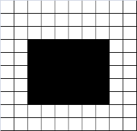
Strel Vertical Strel Square Strel Horizontal Strel Diagonal

Strel Cross

Next the images.

Triangle Square Plus Hollow Square

Now, let us examine what happens when we use a strel to erode the different images. The following pairs are matched as prediction then actual output.

Vertical on Triangle Prediction Vertical on Triangle

Vertical on Square Prediction Vertical on Square

Vertical on Plus Prediction Vertical on Plus

Vertical on Square Prediction Vertical on Square

Square on Triangle Prediction Square on Triangle

Square on Square Prediction Square on Square

Square on Plus Prediction Square on Plus

Square on Hollow Square Prediction Square on Hollow Square

Horizontal on Triangle Prediction Horizontal on Triangle

Horizontal on Square Prediction Horizontal on Square

Horizontal on Plus Prediction Horizontal on Plus

Horizontal on Hollow Square Prediction Horizontal on Hollow Square

Diagonal on Triangle Prediction Diagonal on Triangle

Diagonal on Square Prediction Diagonal on Square

Diagonal on Plus Prediction Diagonal on Plus

Diagonal on Hollow Square Prediction Diagonal on Hollow Square

Cross on Triangle Prediction Cross on Triangle

Cross on Square Prediction Cross on Square

Cross on Plus Prediction Cross on Plus

Cross on Hollow Square Prediction Cross on Hollow Square

We can see that predictions were correct for almost all strel-image pairs. This is due to the adjustment of the center pixels to the (1,1) coordinate rather than the center of the strel for those with even pixel sides. The only problem encountered is the use of diagonal as the strel. The problem is that the error is not symmetric and any logical flipping of the strel does not give out proper results.

Next, we examine the dilation of the images using the different strel. Again, the same change in center pixel is used as in erode.

Vertical on Triangle Prediction Vertical on Triangle

Vertical on Square Prediction Vertical on Square

Vertical on Plus Prediction Vertical on Plus

Vertical on Hollow Square Prediction Vertical on Hollow Square

Square on Triangle Prediction Square on Triangle

Square on Square Prediction Square on Square

Square on Plus Prediction Square on Plus

Square on Hollow Square Prediction Square on Hollow Square

Horizontal on Triangle Prediction Horizontal on Triangle

Horizontal on Square Prediction Horizontal on Square

Horizontal on Plus Prediction Horizontal on Plus

Horizontal on Square Prediction Horizontal on Square

Diagonal on Triangle Prediction Diagonal on Triangle

Diagonal on Square Prediction Diagonal on Square

Diagonal on Plus Prediction Diagonal on Plus

Diagonal on Hollow Square Prediction Diagonal on Hollow Square

Cross on Triangle Prediction Cross on Triangle

Cross on Square Prediction Cross on Square

Cross on Plus Prediction Cross on Plus

Cross on Hollow Square Prediction Cross on Hollow Square

Now, we can see disparities between my predictions and the actual input. But here is the trick. My images were created as large as the defined shapes, no more no less. In dilation, most of the time an increase in the number of pixels of the output. Unfortunately, Scilab does not increase the size of the image. Instead, it crops out the last columns and the last rows until the output image is the same size as the input image. If we examine the predictions, we can see that they predict the output of the function less the last columns and last rows.

Now, let us explore other types of morphological operations. Another pair of morphological operations that will be extremely useful in the future is the Opening and Closing. From their names, they open and close images with holes or discontinuities in them. Or they can join or separate different shapes near each other. The process of Opening and Closing uses both eroding and dilating in different orders. Opening erodes first then dilates while Closing dilates first then erodes. The idea of using both is to change the image then return the regions that are not of interest back to their original state. For example, if we take a annulus and close it, we will result in a circle with the same radius as its outer radius. While if we open it, we will have an annulus with a larger hole inside by same outer radius (granted both opening and closing is dependent on the strel used).

For this exercise I give myself a grade of 9 because of the lateness of my submission. The exploration of how Scilab cuts the image during dilation can be very useful for future exercises.