One very common application of image processing is computing for the area of a certain image. From satellite images to scanning electron microscope images, the use of programming for area calculations can be very useful.
From Physics 112, we know that the area of a certain 2 dimensional shape can be solved using a double integral. But by using Green’s function, we can simplify this integral to a single contour integral by integrating over the contour of the shape.
This concept can be used in programming by digitizing the equation into a summation.
Using this equation, we can easily compute for the area of any figure given certain assumptions, which we will discuss later.
So, let’s start with basic shapes, the rectangle, the triangle and the circle. First we generate the images using Scilab.

Figure 1: Rectangle

Figure 2: Triangle

Figure 3: Circle
1 nx = 500; ny = 500;
2 x_range = linspace(-5,5,nx);
3 y_range = linspace(-5,5,ny);
4 caliby = (max(y_range)-min(y_range))/ny;
5 calibx = (max(x_range)-min(x_range))/nx;
6 y0 = min(y_range);
7 x0 = min(x_range);
8 //Cirlce
9 radius = 3;
10 [X,Y] = ndgrid(x_range,y_range);
11 r= sqrt(X.^2 + Y.^2);
12 A = zeros (nx,ny);
13 A (find(r
14 xset('window',0);
15 imshow (A, []);
16 imwrite (A, 'C:\Users\Amelie\Desktop\Area of defined edges\Circle.bmp');
17 //Triangle
18 hb = 3; hh = 3; slope = -1; y_int = 0;
19 [X,Y] = ndgrid(x_range,y_range);
20 A = ones(nx,ny);
21 A (find(abs(X)>hb)) = 0;
22 A (find(abs(Y)>hh)) = 0;
23 A (find(Y-(slope*X) - y_int >0)) = 0;
24 xset('window',1);
25 imshow (A, []);
26 imwrite (A, 'C:\Users\Amelie\Desktop\Area of defined edges\Triangle.bmp');
27 //Rectangle
28 width = 2; leng = 3;
29 [X,Y] = ndgrid(x_range,y_range);
30 A = ones(nx,ny);
31 A(find(abs(X)>leng)) = 0;
32 A(find(abs(Y)>width)) = 0;
33 xset('window',2);
34 imshow(A, []);
35 imwrite (A, 'C:\Users\Amelie\Desktop\Area of defined edges\Rectangle.bmp');
The circle and rectangle are shapes taken from activity 1, while the triangle is brand new. Basically, to create a triangle, we define the base and height in lines 21 and 22. Then we define the hypotenuse using the equation of a line (line 23). Lines 4 and 5 are used to calculate for the calibration constant (units/pixel). We will use this later to compare the computed area and the theoretical area.
Next, we use the built-in function of Scilab, follow, to find the contour of the shapes. This will create an array of x and y coordinates of the contour itself. By default, it will follow an 8-conectivity rule. Now, since we have the coordinates of the contour, we can iterate the summation in equation 2 to arrive at the value of the calculated area of the shape in terms of pixels. To arrive at the area in Scilab units, we then multiply the x and y coordinates of the contour with the calibration constant. This will now give us the contour and, consequently, the area in terms of Scilab units. Then, by using the defined dimensions of the shape, we can calculate the percent error of each shape.
1 //Rectangle Area Calculations
2 rect = imread('C:\Users\Amelie\Desktop\Area of defined edges\Rectangle.bmp');
3 [x,y] = follow(rect);
4 y = (y.*caliby) + y0;
5 x = (x.*calibx) + x0;
6 x_size = length(x);
7 y_size = length(y);
8 Area = 0;
9 for i = 1:x_size-1;
10 Area = Area + x(i)*y(i+1) - y(i)*x(i+1);
11 end
12 'Rectangular Area'
13 Area = Area/2
14 theo_area = width*2*leng*2
15 percent = abs(Area-theo_area)*100/abs(theo_area)
16 //Triangle Area Calculations
17 tri = imread('C:\Users\Amelie\Desktop\Area of defined edges\Triangle.bmp');
18 [x,y] = follow(tri);
19 y = (y.*caliby) + y0;
20 x = (x.*calibx) + x0;
21 x_size = length(x);
22 y_size = length(y);
23 Area = 0;
24 for i = 1:x_size-1;
25 Area = Area + x(i)*y(i+1) - y(i)*x(i+1);
26 end
27 'Triangular Area'
28 Area = Area/2
29 theo_area = hb*2*hh
30 percent = abs(Area-theo_area)*100/abs(theo_area)
31 //Circle Area Calculations
32 circ = imread('C:\Users\Amelie\Desktop\Area of defined edges\Circle.bmp');
33 [x,y] = follow(circ);
34 y = (y.*caliby) + y0;
35 x = (x.*calibx) + x0;
36 x_size = length(x);
37 y_size = length(y);
38 Area = 0;
39 for i = 1:x_size-1;
40 Area = Area + x(i)*y(i+1) - y(i)*x(i+1);
41 end
42 'Circular Area'
43 Area = Area/2
44 theo_area = %pi*radius^2
45 percent = abs(Area-theo_area)*100/abs(theo_area)
We can see that the program calculated the area of the shapes to as close as 0.95% error. This is extremely accurate considering the loss of information in digitalizing the shape. Also, since the contour is the boundary of the shape and should be included in the area calculation, unlike in the Green’s theorem where the contour is just a series of points that are dimensionless, additional error can be seen.
Rectangular Area
Area = 23.7706
Theoretical Area = 24.
Percent Error = 0.9558333%
Triangular Area
Area = 17.818
Theoretical Area = 18.
Percent Error = 1.0111111%
Circular Area
Area = 27.969
Theoretical Area = 28.274334
Percent Error = 1.0798977%
For simple, continuous shapes, application of the Green’s Theorem is very simple. But one common problem encountered with Green’s Theorem is discontinuity. Green’s theorem is applicable only to contours where the shape inside is continuous. One example of this problem is the annulus.
The annulus is a circular aperture with a circular block in the middle. Calculating the area of the annulus becomes problematic since there is a discontinuity inside. When using the follow function, it will get the contour of the outside circle and disregard the discontinuity inside. To solve this, we take a look at the solutions used when solving discontinuities in paper.
One method is to assume a discontinuous line from the outer circle to the inner circle, take the contour of the new shape, then let the width of the line approach zero. Since we cannot let the line width to approach zero, we make the line as this as possible. Now, if we use the follow function we will get the contour of the annulus with the discontinuity considered.

Figure 4: Annulus

Figure 5: Annulus with line
1 //Annulus
2 outr = 3; inr = 2;
3 [X,Y] = ndgrid(x_range,y_range);
4 r= sqrt(X.^2 + Y.^2);
5 A = zeros (nx,ny);
6 A (find(r
7 A (find(r
8 xset('window',3);
9 imshow (A, []);
10 imwrite (A, 'C:\Users\Amelie\Desktop\Area of defined edges\Annulus.bmp');
11 //Annulus with line
12 [X,Y] = ndgrid(x_range,y_range);
13 r= sqrt(X.^2 + Y.^2);
14 A = zeros (nx,ny);
15 A (find(r
16 A (find(r
17 A (find(abs(X) <>0)) = 0;
18 xset('window',4);
19 imshow (A, []);
20 imwrite (A, 'C:\Users\Amelie\Desktop\Area of defined edges\Annulus with line.bmp');
Annulus Area
Area = 27.969
Theoretical Area = 15.707963
Percent Error = 78.056184%
Annulus with line Area
Area = 15.277
Theoretical Area = 15.707963
Percent Error = 2.7435974%
We can see that the calculations for the annulus area without the line has a 78% error, while with the line comes to a 2.74% error. Also, we can see that the area calculated for the annulus without the line is the same as the area calculated for the circle. This shows that the follow function does not take into consideration the discontinuity of the annulus.
Now, let’s move on to more complicated scenarios. With the improvements in satellite technology, Google Earth has emerged. Satellite images of the whole world are now available online. With this technology, we can now examine parts of the world without actually being there. By using this technology and combining them with our image processing skills, we can find the area of any place we want.
Let us consider an area we know for a fact. So let us examine a house in Casa Milan Neopolitan subdivision in Fairview, Quezon City. We know that one house in this village occupies 300 square meters of lot. So, we can examine the boundaries of the house manipulate the image and get the area of the lot using techniques stated above.
Figure 6: Original Image of a House in Casa Milan
Now, since the image has a blurred boundary and the edge of the house is roughly the same color as that of the background, we need to manipulate the image a bit. We enter the image into paint and outline the boundary with the line tool in paint. Then, we fill the inside with black.

Figure 7: Manipulated Image
Now, we call this image into Scilab and convert it to gray scale and adjust the threshold to get the isolated image. This will give us an image of black with white background. So we need to invert the image.

Figure 8: Gray Scaled Image

Figure 9: Inverted Image
Once we have the inverted image, we can now use the follow function of Scilab and use the same algorithm above to calculate the area of the lot. Now, this will give us the area in terms of pixels. So we find the calibration constant. This can be retrieved using the scale used by Google. From the scale, we use the method used in activity 1 and calculate the number of meters per pixel.

Figure 10: Scale used by Google
1 //Google Map of Casa Milan
2 image = imread('C:\Users\Amelie\Desktop\Area of defined edges\Casa Milan.png');
3 house = im2bw(image,0.01);
4 xset('window',5);
5 imshow(house,2);
6 imwrite(house, 'C:\Users\Amelie\Desktop\Area of defined edges\House converted.bmp');
7 [xcoor,ycoor] = size(house);
8 for i=1:xcoor
9 for j=1:ycoor
10 if house(i,j) == 0 then
11 house(i,j) = 1;
12 else house(i,j) = 0;
13 end
14 end
15 end
16 xset('window',6);
17 imshow(house,2);
18 imwrite (house, 'C:\Users\Amelie\Desktop\Area of defined edges\House inverted.bmp');
19 [x,y] = follow(house);
20 x = (x.*20/69);
21 y = (y.*20/69);
22 x_size = length(x);
23 y_size = length(y);
24 Area = 0;
25 for i = 1:x_size-1;
26 Area = Area + x(i)*y(i+1) - y(i)*x(i+1);
27 end
28 'House in Casa Milan'
29 Area = Area/2
30 theo_area = 300
31 percent = abs(Area-theo_area)*100/abs(theo_area)
From this method we can now arrive at the computed area and the percent difference.
House in Casa Milan
Area = 306.65827
Theoretical Area = 300.
percent = 2.2194217%
From the method used above, we see that a percent error of 2.22% was arrived at. We can now conclude that this method is precise. We can account the error in the definition of the boundary as well as the precision of the image since uploading reduces the quality of the image.
For this activity, I give myself a score of 10. Though I finished the activity and explored the effect of discontinuities in using the follow function, I submitted late hence the bonus I believe I should have gotten should be removed.
I credit the image of the Casa Milan House to Google Earth. And I would like to thank Androphil Polinar, Celestino Borja and Arvin Mabilangan for their comments on style of the presentation.


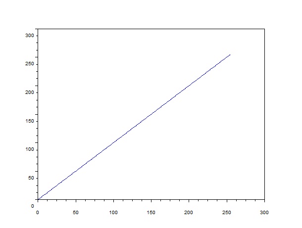
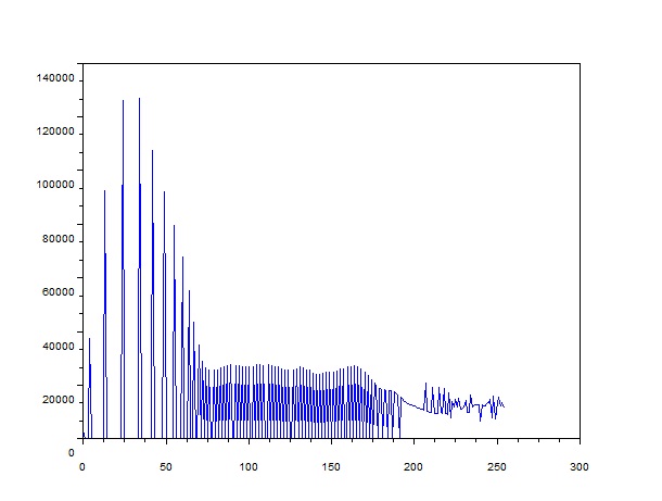


 is used to scale the desired CDF to the original CDF. Then we use the values of the gray scale image to find the corresponding desired gray scale values.