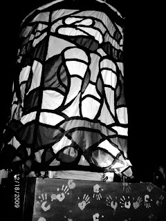
When examining a gray scale image, majority of the pixels will be in between white and black. This is due to the conversion of color to gray scale. It is very difficult to see a truly black color when converting color to gray scale. But this can be adjusted via histogram manipulation.
A histogram of an image will tabulate the number of pixels with the same gray scale value. This will give us the Probability Distribution Function (PDF) or histogram. From the PDF, we can obtain the Cumulative Distribution Function by getting the sum of the PDF as we increase the gray scale value.
By obtaining the CDF of the image we can generate a one to one function that is similar to the original CDF of the image. Then we can backproject the desired CDF function to the original CDF function to vary the gray scale values of the image, and hence manipulate the contrast of the original image.
Let us try to back project using a linear CDF function. First, we get the histogram of the image. We can do this by hacking the histplot function of Scilab to return the values of the histogram. Next, we get the CDF of the histogram by using the cumsum function. Now, since we are back projecting a linear plot, we know that if the slope is 1 and y intercept is 0, the value of the cumsum function should be the gray scale value of that pixel. So by using the following equation,
and run it for all pixels of the image, we can back project a linear CDF function to the image.
Figure 1: Original Image
Figure 2: Original Probability Distribution Function
Figure 3: Original Cumulative Distribution Function
Figure 4: Linear Cumulative Distribution Function
Figure 5: Probability Distribution Function Post Processing for Linear Back Projecting
Figure 6: Cumulative Distribution Function Post Processing for Linear Back Projecting
Figure 7: Processed Image Using Linear Cumulative Distribution Function
We can see the effect of the process through figures 1 to 7. We can see that the image brightens but does not improve the contrast. When we examine original CDF, we can see a natural logarithmic trend. So what will happen to the image if we use a natural logarithmic CDF to smoothen the CDF?
To do this, we need to use a little more complicated method than the previous steps. First, we create a logarithmic plot. Now, we need to find the corresponding gray value that we will back project to the original image. To do so, we use the following equation,
where ysum is the y-axis of the original CDF and ysum2 is the y-axis values of the desired CDF. This equation is derived from the equation of the desired CDF. The  is used to scale the desired CDF to the original CDF. Then we use the values of the gray scale image to find the corresponding desired gray scale values.
Figure 8: Logarithmic Cumulative Distribution Function
Figure 9: Probability Distribution Function Post Processing for Logarithmic Back Projecting
Figure 10: Cumulative Distribution Function Post Processing for Logarithmic Back Projecting
Figure 11: Processed Image Using Logarithmic Cumulative Distribution Function
We can see that the contrast is tons better. The gray areas in the middle of the lantern became white while the black borders became darker. Also, we can see that the hand prints on the base of the lantern stands out more.
Though this method is very objective, most image processing programs have the option of adjusting the curves at which back projecting happens. One of the image processing programs available online is GIMP. Though instead of using the cumulative distribution function, it uses an x-y plot where the x-axis is the gray scale value of the original image while the y-axis is the gray scale value you will back project to the image. Now, on the plot is a line that you can adjust. By following the x-axis and the corresponding y-axis values of the line, you will find the values you need to back project.
Figure 12: Original GIMP Gray Scale Image
Figure 13: Curve Adjustment Option for GIMP
Figure 14: Zoomed GIMP Edited Image
We can see, when comparing the processed image using logarithmic CDF and the GIMP edited image, that both images have highly improved contrast. We can see that both methods have benefits. The GIMP image has the benefit of being highly flexible as adjusting the curve adjusts the image immediately. The problem is that it is highly subjective. Adjustments in the curve leave only human judgment on improvements to the image. In comparison, using the CDF back projecting method has the benefit of viewing the graphs of the CDF. Smoothening of the CDF usually improves contrast and image quality. But using this method needs several steps to see the correlation of the CDF and the back projecting gray scale values.
For this activity, I give myself a score of 8. Though I finished the activity, I submitted late so I believe the deduction of 2 points is just.
I would like to thank Melissa Dy of the 09-10 College of Science Student Council for the picture of the CS Lantern. And Celestino Borja, Androphil Polinar and Arvin Mabilangan for their comments on style of the presentation.


No comments:
Post a Comment